Machine Learning: Building Our First Classifier with Scikit-Learn

In this lab, we roll up our sleeves and train our very first machine learning model using Scikit-Learn... a staple in the data science toolkit. We dive into the Iris dataset, use a K-Nearest Neighbours (KNN) classifier, and explore how to measure performance through accuracy, confusion matrices, and cross-validation.

Lab Objectives

Okay, for this lab I wanted to understand and remind myself how traditional machine learning techniques worked so the goals is to:

• Load and inspect a labelled dataset
• Split data for training and testing
• Train a classical ML model (KNN)
• Evaluate predictions with performance metrics
• Visualise results and understand model behaviour

Dataset: The Iris Classic

We're working with the Iris dataset; a clean, structured dataset with 150 flower samples across 3 classes: setosa, versicolor, and virginica

Each sample has 4 numerical features:

• Sepal length & width
• Petal length & width

The simplicity and balance of this dataset make it ideal for our first classification experiment.

If you've never studied botany, the terms in the Iris dataset might feel abstract.

• Sepals are the outer, leaf-like parts of a flower; they protect the bud before it opens. These often curve downward (called falls)
• Petals are the colourful inner parts; designed to attract pollinators. These stand upright (called standards)

These four features give the model a surprisingly clear picture of species differences and it's why KNN performs so well here.

What Is K-Nearest Neighbours (KNN)?

K-Nearest Neighbours, or KNN for short, is one of the simplest and most intuitive algorithms in machine learning. It's a great starting point for understanding how classification works... and while it may be simple, it can be remarkably effective, especially on clean datasets like the Iris flower set.

At its core, KNN is a type of instance-based learning. It doesn't build a traditional predictive model during training. Instead, it stores all the training data and makes predictions only when needed... which is why it's often called a lazy learner. When asked to classify a new input, it compares that input to the training examples and finds the 'k' closest neighbours based on distance (typically using Euclidean distance). The predicted class is simply the one most commonly represented among those neighbours.

For example, imagine we're trying to classify a new flower. KNN would look at its sepal and petal dimensions, then find the three or five closest flowers from the training set. If most of those neighbours are labelled "setosa" that's what the algorithm will predict.

Lab Breakdown

Here's the flow of what we built in terms of our lab code and some of the outputs we received:

1. Load the Data - Pulled in via load_iris() and converted to Pandas for inspection

iris = load_iris()
X = pd.DataFrame(iris.data, columns=iris.feature_names)
y = pd.Series(iris.target, name="species")

print(X.head())
print(y.head())

$ python lab02.py
   sepal length (cm)  sepal width (cm)  petal length (cm)  petal width (cm)
0                5.1               3.5                1.4               0.2
1                4.9               3.0                1.4               0.2
2                4.7               3.2                1.3               0.2
3                4.6               3.1                1.5               0.2
4                5.0               3.6                1.4               0.2
0    0
1    0
2    0
3    0
4    0
Name: species, dtype: int64

2. Split the Data - Used train_test_split() to allocate 80% for training and 20% for testing

X_train, X_test, y_train, y_test = train_test_split(
    X, y, test_size=0.2, random_state=42
)

3. Train the Model - Fitted the KNN model to the training set i.e. use 80% of the iris training data and feed it into model

model = KNeighborsClassifier(n_neighbors=3)
model.fit(X_train, y_train)

4. Validate the model - Produce an accuracy score based on predictions

y_pred = model.predict(X_test)
print(f"Accuracy: {accuracy_score(y_test, y_pred):.2f}")

The accuracy calculation is basically number of correct predictions) / total number of predictions For our dataset, this accuracy rating is a solid metric because every class has roughly the same number of samples, if the data was significantly weighted towards a particular class then accuracy alone probably isn't the right metric to validate the model with.

5. Evaluate Performance - Used accuracy_score, confusion_matrix, and classification_report to measure accuracy and diagnose model behaviour

# Confusion Matrix
cm = confusion_matrix(y_test, y_pred)
sns.heatmap(cm, annot=True, fmt='d', cmap='Blues')
plt.title("Predicted vs Actual")
plt.xlabel("Predicted")
plt.ylabel("Actual")
plt.savefig('predicated-vs-actual.png')
plt.close()

# Classification Report
print(classification_report(y_test, y_pred, target_names=iris.target_names))

What we got for our particular test was:

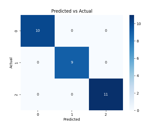
From the diagonals (0, 0), (1, 1), (2, 2) we see that all the data was successfully predicted based on the classification expected. The classification report looks as follows:

              precision    recall  f1-score   support

      setosa       1.00      1.00      1.00        10
  versicolor       1.00      1.00      1.00         9
   virginica       1.00      1.00      1.00        11

    accuracy                           1.00        30
   macro avg       1.00      1.00      1.00        30
weighted avg       1.00      1.00      1.00        30

This tells us the model didn’t just achieve 100% accuracy — it also got a perfect score across all other key metrics:

• Precision: How many predicted labels were correct
• Recall: How many true labels were correctly identified
• F1-Score: The harmonic mean of precision and recall

Given the balanced dataset and the model's strong predictions across all three classes, these scores confirm the KNN model performed flawlessly when predicting the species of a plant based on the petal or sepal measurements (gotta love perfect datasets).

6. Cross-Validate - Used cross_val_score for a more robust estimate of performance across folds

scores = cross_val_score(model, X, y, cv=5)
print(f"Cross-Validation Accuracy: {scores.mean():.2f}")

So with this, we split the data into 5 chunks. Train the model on 4 chunks, test it on the 1 left out... repeating this 5 times so each chunk gets to be the test set once.

In a nutshell... this is a 5-fold cross-validation and it helps us to cross-check that the original 80:20% split wasn't a fluke or happy coincidence, in essence it gives us:

• A more reliable estimate of how your model might perform on new data
• A way to spot overfitting or data leakage if your test scores vary wildly between folds

From our script, this produced a Cross-Validation Accuracy score of 0.97 which given we're using a KNN model and the dataset being used is built specifically for learning (is there such a thing as a perfect dataset??? 😆) indicates that our model is great at predicting plant species based on the dimensions of a sepal or petal.

We'll look at more complex evaluation methods like precision and recall in a future lab, but for now, accuracy is more than enough to show KNN performs brilliantly here.

With perfect scores across the board, this lab showcases just how powerful even the simplest algorithms can be... especially when paired with clean, well-structured data or perfect data in this case 😍

Extending this lab

• Swap in different classifiers like DecisionTreeClassifier or RandomForestClassifier
• Apply feature scaling using StandardScaler
• Use GridSearchCV to optimise n_neighbors for KNN

How to Run It

Clone the repo or copy the files and run:

cd kelcode-ai-labs/02-classical-machine-learning
python -m venv .venv
source .venv/bin/activate

pip install -r requirements.txt
python lab02.py

Outputs:

• predicated-vs-actual.png: Confusion matrix heatmap
• Printed performance metrics

Next Time: Fine-Tuning BERT for Text Classification

In the next lab, we’ll leave the world of flowers behind and step into natural language processing. You’ll train a text classification model using BERT on the AG News dataset, one of the most widely used benchmarks for text-based machine learning.

We'll explore:

• How to load and preprocess text for Transformers
• The steps involved in fine-tuning a pretrained BERT model
• How to evaluate model performance on news headlines
• And how to save your trained model for future use

If you've ever wondered how modern AI systems categorise articles, tweets, or product reviews... this is where it all begins.