Embarking on an AI Engineering Journey: From Data to Deployment

Artificial Intelligence has become ubiquitous, powering everything from personalised recommendations to advanced medical diagnostics. Yet, behind these seamless experiences lie sophisticated engineering practices, robust data science methodologies, and careful deployment strategies. After years spent building platforms, deploying infrastructure, and fine-tuning models, I'm excited to share a structured journey towards mastering AI engineering!

What's the Plan?

I'll be documenting a practical, structured exploration of AI engineering through hands-on labs, clearly explained and reproducible via code hosted on GitHub. We'll begin from foundational concepts, progressively delving into more complex topics... ensuring clarity and practical understanding every step of the way.

Modules Overview

• Module 1: Foundations of AI Modelling (coming soon)
  Setting the stage by understanding essential AI lifecycle concepts and the modern tooling landscape
• Module 2: Data Science & Modelling
  Deep dive into cleaning data, classical machine learning, deep learning fundamentals, advanced optimisation techniques (including LoRA and quantisation), model evaluation, and debugging
• Module 3: AI Engineering & Deployment (Coming Soon)
  Learn packaging, deployment, monitoring, and management of AI models in production environments; from simple APIs to robust Kubernetes deployments
• Module 4: Advanced AI Platform Architecture (Coming Soon)
  Explore cutting-edge concepts such as Retrieval Augmented Generation (RAG), platform scalability, security, and governance

GitHub Repository: kelcode-ai-labs

All labs and experiments will be openly shared and regularly updated in the structured GitHub repository:

kelcode-ai-labs/
├── data-science-track/
│   ├── lab01-data-exploration/
│   ├── lab02-classical-ml/
│   ├── lab03-deep-learning/
│   ├── lab04-model-optimisation/
│   ├── lab05-evaluation-metrics/
│   ├── lab06-model-debugging/
│   └── lab07-quality-improvement/
└── ai-engineering/ (future)

Lab 1 - Data Exploration & Cleaning

Our journey kicks off by mastering core data skills... often the unsung heroes of successful AI work. In Lab 1, we'll dive into why data quality matters, using Python and Pandas to clean and explore a real‑world dataset so it’s ready for deeper analysis and actionable insights.

Lab Objectives

For this particular lab, what I wanted to get out of it was to simply kick off the journey with something simple ...

• Inspect raw data for quality and quirks
• Document and justify each cleaning decision
• Visualise key patterns to guide downstream modelling
• Produce a clean CSV ready for analysis

Initial Inspection

import pandas as pd

df = pd.read_csv('students.csv')
print(df.head())
print(df.info())

$ python lab01.py
<class 'pandas.core.frame.DataFrame'>
RangeIndex: 100 entries, 0 to 99
Data columns (total 9 columns):
 #   Column             Non-Null Count  Dtype
---  ------             --------------  -----
 0   student_id         100 non-null    object
 1   name               100 non-null    object
 2   gender             100 non-null    object
 3   age                48 non-null     float64
 4   major              100 non-null    object
 5   gpa                100 non-null    float64
 6   credits_completed  57 non-null     float64
 7   attendance_rate    48 non-null     float64
 8   country            100 non-null    object
dtypes: float64(4), object(5)
memory usage: 7.2+ KB


Columns: ['student_id', 'name', 'gender', 'age', 'major', 'gpa', 'credits_completed', 'attendance_rate', 'country']
Unique Genders: ['F' 'M']
Score range: 1.21 - 4.0

Quick look at row counts, data types, and missing‑value patterns, what I observed was:

• age and credits_completed have >50% missing
• attendance_rate has sporadic gaps (approx. 43% missing)
• gpa present but varying precision

Cleaning Decisions & Rationale

Cleaning the data is pretty simple with pandas and can be done with a single line for our 2 replacements...

# Apply cleaning steps
df['attendance_rate'] = df['attendance_rate'].fillna(0)
df['gpa'] = df['gpa'].round(2)

Exploratory Visualisations

Now there's a solid understanding of the data we can run a few analyses against it to understand the dataset as a whole a bit better.

The first of these is to create a distribution / trend for the GPA results, code wise we can leverage the seaborn and matplot python libs as follows:

import seaborn as sns
import matplotlib.pyplot as plt

sns.histplot(df['gpa'], kde=True)
plt.title("GPA Distribution")
plt.savefig('gpa-distribution.png')

This produces the following saved image ... pretty cool for 3 lines of code 😆

Next up we can plot the attendance rate against the GPA to see if there is a correlation between them... again a few lines allows us to visualise this:

sns.scatterplot(x='attendance_rate', y='gpa', data=df)
plt.title("Attendance Rate vs GPA")
plt.savefig('attendance-vs-gpa.png')

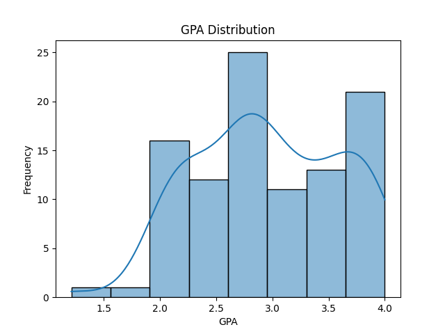
From the histogram (Figure 1), we observe that student GPAs form a rough bell‑shaped curve centred just below 3.0:

• Most students cluster between 2.5 and 3.5 which suggests a moderately high overall performance level
• Slight left skew (skewness ≈ -0.10) indicates a few lower‑performing outliers dragging the tail down, but the bulk remains centred around the mean (≈ 2.96)
• Light tails (kurtosis ≈ -0.83) imply fewer extreme GPAs than a normal distribution would predict... most students fall near the centre of the range

Overall, the GPA distribution looks fairly normal, with most students performing in a tight band and only a handful at the very low end.

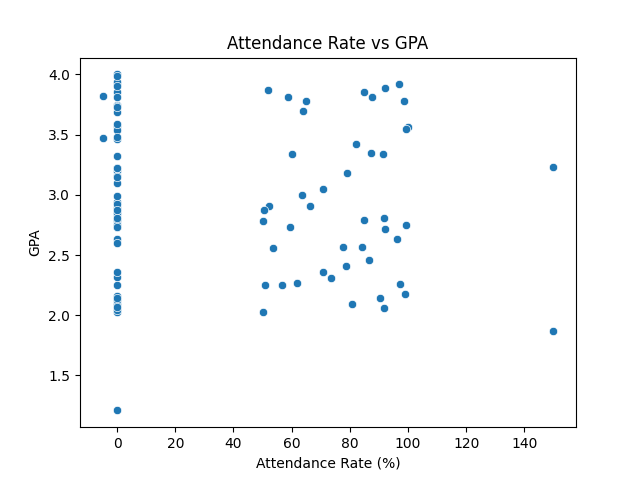
The scatter plot (Figure 2) and the Pearson correlation (r ≈ –0.07) reveal:

• No strong linear relationship: The near‑zero correlation coefficient shows that attendance rate alone doesn’t predict GPA in this dataset.
• Notable outliers: A few students have high GPAs despite very low attendance, and others attend frequently but don’t achieve top grades.
• Potential non‑linear factors: Since attendance doesn’t explain much variance in GPA, other variables (like study habits, prior knowledge, or course difficulty) are likely more influential.

In short, while good attendance is often assumed to boost academic performance, our data shows that, for this cohort, attendance rate isn’t a reliable standalone predictor of GPA, mainly because of the missing data but also it's synthetic data so unlikely to reflect true reality of student achievements...

Potential Extensions

Potential future explorations include examining relationships between credits completed and GPA, performing deeper demographic analyses, and preparing data for predictive modelling.

Running the Lab:

Setup requires Python 3.11.2 and can be done by running:

cd data-science-track/01-data-exploration
python -m venv .venv
source .venv/bin/activate
pip install -r requirements.txt
python lab01.py

If you don't run a venv you can simply run:

cd data-science-track/01-data-exploration
pip install -r requirements.txt
python lab01.py

NB: Results (CSV files and visualisation PNGs) are generated automatically.

Next Time

Next time, we’ll dive into Lab 2: Classical Machine Learning, exploring how to load, split, train, and evaluate a classifier using pandas and Scikit‑Learn.

If you found this kickoff useful, feel free to ⭐ star the GitHub repo at kelcode‑ai‑labs. See you in the next lab!