Fine-Tuning a Model with LoRA

Previously, we learned how to train a BERT model with the AG News dataset and how to interact with our new model as part of the evaluation process. A natural continuation of this is to extend our model with some new categories and extend the capabilities of the model.

To start training our model, we need to look at combining the labels in use i.e. the ones the model has already been trained with World, Sports, Business, Sci/Tech and include our own categories for climate, education, health, security and tech-policy.

This allows us to categorise headlines like UK health service braces for record winter surge as a more fitting "health" category instead of the typical "business" or "world" categories.

What is LoRA?

Low-Rank Adaptation or LoRA for short is a parameter-efficient fine-tuning technique that injects small, trainable "adapter" matrices into select weight-blocks of a pre-trained model... most commonly the attention query and value projections.

To put it simply... we can think of our big pre-trained model as a massive encyclopedia that we don't want to rewrite. LoRA is like taping in a handful of sticky notes where you jot down updates for your new topic. You leave the original encyclopedia pages untouched and only train those tiny sticky notes. This way we can teach it something new without having to reprint the whole thing... saving a ton of time, memory, and compute.

Sooooo instead of updating all ~110 million parameters, LoRA freezes the original weights and learns only these low-rank adapters (e.g. rank r = 8), which typically amount to less than 1% of the model’s total parameters. This dramatically cuts GPU memory and compute costs while still allowing the model to adapt fully to your downstream task.

Prepare the dataset

To train our model with our own categories, we need to prep some data that we can use for training our model.

Our dataset basically needs to consist of 2 elements:

1. Headline - The news headline related to the label we want to train
2. Label - one of our labels previously defined

For the purpose of this lab, we'll get AI to generate it and the script I used to generate this data will be included into the code repo for this lab but in essence it gives us 10k rows that look like the following:

"text","label"
"UK Government to Invest in New Border Control Measures","security"
"UK's vaccine rollout hailed as 'remarkable achievement' but concerns over distribution persist","health"
"Climate-related wildfires ravage the UK, leaving hundreds displaced and homes destroyed","climate"
"GPs call for more resources to tackle rising demand","health"
"New study reveals link between diet and mental health.","health"
"UK Government Introduces New Laws to Strengthen Cyber Security","security"
...
...

Now we have our dataset, it's time to put it to use🤘

# Step 1 - Load and prepare the dataset
# Load AG News
ag_dataset = load_dataset("ag_news", split="train")
ag_df = pd.DataFrame({
  "text": ag_dataset["text"],
  "label": ag_dataset["label"]
})

# Map AG News labels to strings
ag_df["label"] = ag_df["label"].map({
  0: "World",
  1: "Sports",
  2: "Business",
  3: "Sci/Tech"
})

# Load custom dataset
uk_df = pd.read_csv("synthetic_news_uk.csv")
uk_df = uk_df.rename(columns={"label": "label", "text": "text"})

# Combine datasets
combined_df = pd.concat([ag_df, uk_df], ignore_index=True)
dataset = Dataset.from_pandas(combined_df)

# Encode labels
label_encoder = LabelEncoder()
label_encoder.fit(dataset["label"])
dataset = dataset.map(lambda x: {"label": x["label"]})
dataset = dataset.map(lambda x: {"labels": label_encoder.transform([x["label"]])[0]})

This snippet basically builds up the labels from both the AG News dataset and our synthetic dataset. We then encode the labels into a contiguous range of integer values and load them into the dataset.

Train the model

Now we've prepped our dataset it's time to do some training ... this may take a while.

# Load tokenizer
lab03_model_path = str(Path("../../03-deep-learning/lab03-model").resolve())
tokenizer = AutoTokenizer.from_pretrained(lab03_model_path, local_files_only=True)

# Tokenise
def tokenize(data):
  return tokenizer(data["text"], padding="max_length", truncation=True, max_length=128)

dataset = dataset.map(tokenize, batched=True)
dataset.set_format(type="torch", columns=["input_ids", "attention_mask", "labels"])
dataset = dataset.train_test_split(test_size=0.2, seed=42, shuffle=True)
train_data = dataset["train"]
eval_data = dataset["test"]

# Load base model
model = AutoModelForSequenceClassification.from_pretrained(
  lab03_model_path,
  num_labels=len(label_encoder.classes_),
  ignore_mismatched_sizes=True,
  local_files_only=True,
  use_safetensors=True
)

# Configure LoRA
lora_config = LoraConfig(
  r=8,
  lora_alpha=32,
  target_modules=["query", "value"],
  lora_dropout=0.1,
  bias="none",
  task_type=TaskType.SEQ_CLS,
)
model = get_peft_model(model, lora_config)
model.print_trainable_parameters()

# Train
training_args = TrainingArguments(
  output_dir="lora-news/",
  per_device_train_batch_size=16,
  per_device_eval_batch_size=16,
  num_train_epochs=5,
  learning_rate=2e-4,
  evaluation_strategy="epoch",
  save_strategy="epoch",
  logging_dir="./logs",
  logging_steps=10,
  report_to="none"
)

trainer = Trainer(
  model=model,
  args=training_args,
  train_dataset=train_data,
  eval_dataset=eval_data,
)

trainer.train()
print("✅ Training complete!")

Okay, so there's a lot of code here but's not actually that complicated... let's break it down:

1. Local checkpoint loading: Pull in a pre-trained tokenizer and sequence-classification model from our previous lab session, automatically adjusting the head to match the number of labels we're using (9 in total)
2. Efficient data prep: Batch-tokenise the texts to a fixed length of 128 tokens i.e. pad/truncate¹ each headline before converting everything into PyTorch tensors, then we shuffle and split the dataset into an 80/20 train/eval split
3. Configure LoRA: Rather than updating all ~110 million parameters, wrap the model with low-rank adapters (r=8) focusing on the "query" and "value" layers. This freezes the bulk of the model and trains only a tiny fraction of new weights
4. Standard HF Trainer setup: Setup the training args (batch size 16, 5 epochs, LR 2e-4, eval & save each epoch), hook up the LoRA-enabled model and datasets to Trainer, then call .train()

¹Unlikely to truncate our text here as we're only dealing with headlines so it's more likely to be padded with zeros

As it's running, you see a screen full of:

{'loss': 0.0578, 'grad_norm': 0.4387788772583008, 'learning_rate': 0.00018775384615384616, 'epoch': 0.31}
{'loss': 0.0822, 'grad_norm': 0.35523760318756104, 'learning_rate': 0.0001876923076923077, 'epoch': 0.31}
{'loss': 0.0709, 'grad_norm': 0.11925731599330902, 'learning_rate': 0.00018763076923076924, 'epoch': 0.31}
{'loss': 0.082, 'grad_norm': 7.286395072937012, 'learning_rate': 0.0001875692307692308, 'epoch': 0.31}
{'loss': 0.039, 'grad_norm': 0.008671889081597328, 'learning_rate': 0.00018750769230769233, 'epoch': 0.31}
{'loss': 0.0243, 'grad_norm': 2.4974987506866455, 'learning_rate': 0.00018744615384615386, 'epoch': 0.31}
{'loss': 0.0279, 'grad_norm': 0.026241207495331764, 'learning_rate': 0.0001873846153846154, 'epoch': 0.32}
{'loss': 0.0725, 'grad_norm': 0.051251377910375595, 'learning_rate': 0.00018732307692307694, 'epoch': 0.32}
{'loss': 0.0201, 'grad_norm': 0.7329538464546204, 'learning_rate': 0.00018726153846153847, 'epoch': 0.32}
{'loss': 0.0461, 'grad_norm': 0.07000083476305008, 'learning_rate': 0.00018720000000000002, 'epoch': 0.32}
{'loss': 0.0129, 'grad_norm': 0.1153610423207283, 'learning_rate': 0.00018713846153846155, 'epoch': 0.32}

This is basically the logs from the Hugging Face Trainer as per the logging_steps setting we defined in the training_args. Each line basically shows:

• loss: the average prediction from the batch about how wrong the model is, lower the better here...
• grad_norm: the ℓ₂‐norm of the gradients (a rough gauge of update magnitude)
• learning_rate: the current LR for the epoch batch
• epoch: how far you are into the current epoch (e.g. 0.31 means 31% through epoch 1)

After a while (about 20 mins on my rig), you'll see the final training report which basically tells us how long training took, how fast it ran, and what the final average loss was.

{'train_runtime': 1280.2465, 'train_samples_per_second': 406.172, 'train_steps_per_second': 25.386, 'train_loss': 0.03426654428535392, 'epoch': 5.0}
100%|█████████████████████████████████████████| 32500/32500 [21:20<00:00, 25.39it/s]
✅ Training complete!

In our case, the total run took 21 minutes, it trained 406 rows per second, executed 25 optimisation steps (batches) per second and resulted in a loss factor of 0.0343 which is incredibly low and means our model is pretty confident in its ability to categorise headlines across all 9 categories.

Evaluating the model

Now we have our finished model it's time to evaluate it's effectiveness...

predictions = trainer.predict(eval_data)
preds = torch.argmax(torch.tensor(predictions.predictions), dim=1).numpy()
true = predictions.label_ids

pred_labels = label_encoder.inverse_transform(preds)
true_labels = label_encoder.inverse_transform(true)

print("Evaluation Results")
print(f"Accuracy: {accuracy_score(true_labels, pred_labels):.4f}")
print("\nClassification Report:")
print(classification_report(true_labels, pred_labels, target_names=label_encoder.classes_))

# Confusion matrix
cm = confusion_matrix(true_labels, pred_labels, labels=label_encoder.classes_)
plt.figure(figsize=(10, 8))
sns.heatmap(cm, annot=True, fmt="d", cmap="Blues", xticklabels=label_encoder.classes_, yticklabels=label_encoder.classes_)
plt.xlabel("Predicted Label")
plt.ylabel("True Label")
plt.title("Confusion Matrix")
plt.tight_layout()
plt.savefig("confusion_matrix_9class.png")
plt.close()

# Save merged model
merged_model = model.merge_and_unload()
label2id = {label: i for i, label in enumerate(label_encoder.classes_)}
id2label = {i: label for label, i in label2id.items()}
merged_model.config.label2id = label2id
merged_model.config.id2label = id2label

merged_model.save_pretrained("lora-news/full-model")
tokenizer.save_pretrained("lora-news/full-model")
model.save_pretrained("lora-news/adapter")

print(f"\n✅ Model and tokenizer saved to 'lora-news/'")

For the models, we save the full LoRA-trained model and the adapters from each epoch so we can do something with them in the subsequent labs.

Similar to previous labs, we'll leverage the confusion matrix and classification reports to determine how well our model is working with our new labels and synthetic dataset.

This gives us the following outputs:

Accuracy: 0.9906

Classification Report:
              precision    recall  f1-score   support

    Business       0.99      0.99      0.99      5992
    Sci/Tech       0.99      0.99      0.99      5940
      Sports       1.00      1.00      1.00      6068
       World       0.99      0.99      0.99      6041
     climate       0.96      0.98      0.97       368
   education       0.99      0.98      0.98       370
      health       0.98      0.98      0.98       417
    security       0.95      0.96      0.95       409
 tech-policy       0.95      0.95      0.95       395

    accuracy                           0.99     26000
   macro avg       0.98      0.98      0.98     26000
weighted avg       0.99      0.99      0.99     26000

So we can interpret these results as follows:

• Accuracy: On your 26 000 held-out examples, the model got about 99.06% of them exactly right
• Weighted avg F1-score: Since our big "Business", "Sci/Tech", "Sports" and "World" classes dominate the data, the weighted average is nearly the same as overall accuracy
• Macro avg F1-score: Averaging F1 scores equally across all 9 classes gives us about 0.98 which still excellent, but it highlights that the smaller, "synthetic" classes (climate, education, health, security, tech-policy) have a slightly lower performance than the original four which given there are fewer samples to learn from is to be expected

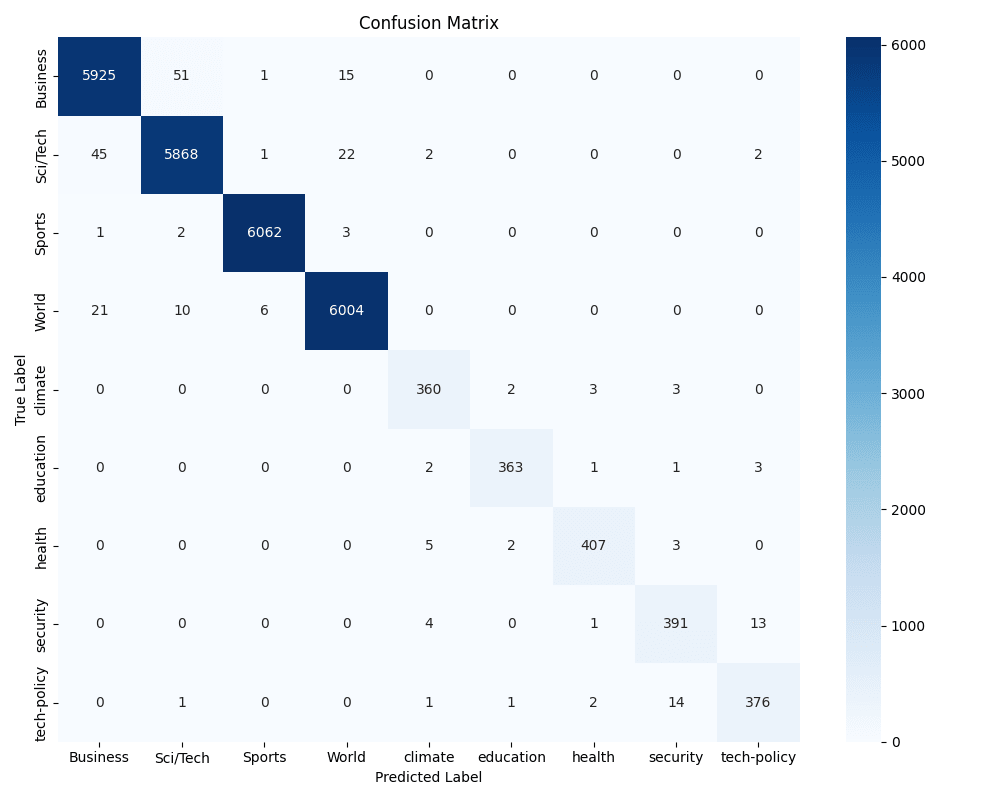
Based on the confusion matrix, we can see that:

• Climate occasionally confuses with education or health (a few mis‐labels among those three)
• Security and tech-policy also get muddled with each other on a handful of samples which semantically makes sense as these topics are more likely to overlap that say "Business" and "Sports"

In a nutshell... our LoRA-fine-tuned BERT model is nailing the four big news categories and doing a very good job on the five new ones too with an overall 99% accuracy and F1 score. A bit more data or targeted tuning on the smallest classes could push this even higher i.e. 5k per new category instead of about 1,600 would make a significant difference.

Next steps

Next up is to quantise our model which makes it significantly smaller and allows us to deploy it as a service... see you next time!